Warning
This is the state of the documentation before this module was moved to the attic. It is likely that code examples shown here do not work as advertised. If you would like to take on any code, you are welcome to its documentation.
New in version 1.6.
This document describes tools in yt for analyzing star particles. The Star Formation Rate tool bins stars by time to produce star formation statistics over several metrics. A synthetic flux spectrum and a spectral energy density plot can be calculated with the Spectrum tool.
This tool can calculate various star formation statistics binned over time.
As input it can accept either a yt data_source, such as a region or
sphere, or arrays containing the data for the stars you wish to analyze.
This example will analyze all the stars in the volume:
import yt
from yt.analysis_modules.star_analysis.api import StarFormationRate
ds = yt.load("Enzo_64/DD0030/data0030")
ad = ds.all_data()
sfr = StarFormationRate(ds, data_source=ad)
or just a small part of the volume i.e. a small sphere at the center of the simulation volume with radius 10% the box size:
import yt
from yt.analysis_modules.star_analysis.api import StarFormationRate
ds = yt.load("Enzo_64/DD0030/data0030")
sp = ds.sphere([0.5, 0.5, 0.5], 0.1)
sfr = StarFormationRate(ds, data_source=sp)
If the stars to be analyzed cannot be defined by a data_source, YTArrays can
be passed. For backward compatibility it is also possible to pass generic numpy
arrays. In this case, the units for the star_mass must be in
\((\mathrm{\rm{M}_\odot})\), the star_creation_time in code units, and
the volume must be specified in \((\mathrm{\rm{Mpc}})\) as a float (but it
doesn’t have to be correct depending on which statistic is important).
import yt
from yt.analysis_modules.star_analysis.api import StarFormationRate
from yt.data_objects.particle_filters import add_particle_filter

def Stars(pfilter, data):
      return data[("all", "particle_type")] == 2
add_particle_filter("stars", function=Stars, filtered_type='all',
                    requires=["particle_type"])

ds = yt.load("enzo_tiny_cosmology/RD0009/RD0009")
ds.add_particle_filter('stars')
v, center = ds.find_max("density")
sp = ds.sphere(center, (50, "kpc"))

# This puts the particle data for *all* the particles in the sphere sp
# into the arrays sm and ct.
mass = sp[("stars", "particle_mass")].in_units('Msun')
age = sp[("stars", "age")].in_units('Myr')
ct = sp[("stars", "creation_time")].in_units('Myr')

# Pick out only old stars using Numpy array fancy indexing.
threshold = ds.quan(100.0, "Myr")
mass_old = mass[age > threshold]
ct_old = ct[age > threshold]

sfr = StarFormationRate(ds, star_mass=mass_old, star_creation_time=ct_old,
                        volume=sp.volume())
To output the data to a text file, use the command .write_out:
sfr.write_out(name="StarFormationRate.out")
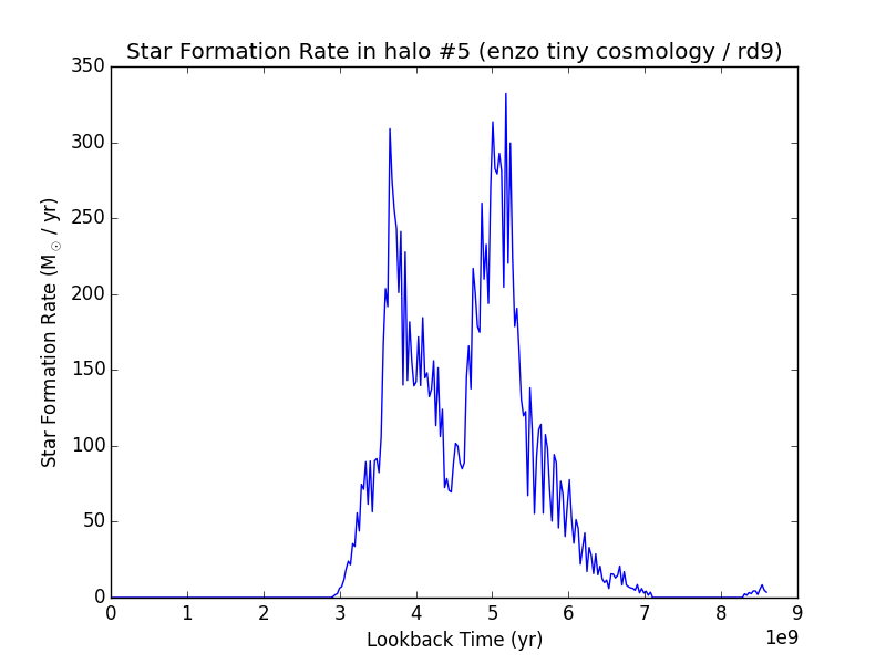
In the file StarFormationRate.out, there are seven columns of data:
- Time (yr)
- Look-back time (yr)
- Redshift
- Star formation rate in this bin per year \((\mathrm{\rm{M}_\odot / \rm{yr}})\)
- Star formation rate in this bin per year per Mpc**3 \((\mathrm{\rm{M}_\odot / \rm{h} / \rm{Mpc}^3})\)
- Stars formed in this time bin \((\mathrm{\rm{M}_\odot})\)
- Cumulative stars formed up to this time bin \((\mathrm{\rm{M}_\odot})\)
The output is easily plotted. This is a plot for some test data (that may or may not correspond to anything physical) using columns #2 and #4 for the x and y axes, respectively:
It is possible to access the output of the analysis without writing to disk.
Attached to the sfr object are the following arrays which are identical
to the ones that are saved to the text file as above:
sfr.timesfr.lookback_timesfr.redshiftsfr.Msol_yrsfr.Msol_yr_volsfr.Msolsfr.Msol_cumulative
Based on code generously provided by Kentaro Nagamine <kn@physics.unlv.edu>, this will generate a synthetic spectrum for the stars using the publicly-available tables of Bruzual & Charlot (hereafter B&C). Please see their 2003 paper for more information and the main data distribution page for the original data. Based on the mass, age and metallicity of each star, a cumulative spectrum is generated and can be output in two ways, either raw, or as a spectral energy distribution.
This analysis toolkit reads in the B&C data from HDF5 files that have been converted from the original ASCII files (available at the link above). The HDF5 files are one-quarter the size of the ASCII files, and greatly reduce the time required to read the data off disk. The HDF5 files are available from the main yt website here. Both the Salpeter and Chabrier models have been converted, and it is simplest to download all the files to the same location. Please read the original B&C sources for information on the differences between the models.
In order to analyze stars, first the Bruzual & Charlot data tables need to be
read in from disk. This is accomplished by initializing SpectrumBuilder and
specifying the location of the HDF5 files with the bcdir parameter.
The models are chosen with the model parameter, which is either
“chabrier” or “salpeter”.
import yt
from yt.analysis_modules.star_analysis.api import SpectrumBuilder
ds = yt.load("enzo_tiny_cosmology/RD0009/RD0009")
spec = SpectrumBuilder(ds, bcdir="bc", model="chabrier")
In order to analyze a set of stars, use the calculate_spectrum command.
It accepts either a data_source, or a set of YTarrays with the star
information. Continuing from the above example:
v, center = ds.find_max("density")
sp = ds.sphere(center, (50, "kpc"))
spec.calculate_spectrum(data_source=sp)
If a subset of stars are desired, call it like this:
from yt.data_objects.particle_filters import add_particle_filter

def Stars(pfilter, data):
    return data[("all", "particle_type")] == 2
add_particle_filter("stars", function=Stars, filtered_type='all',
                    requires=["particle_type"])

# Pick out only old stars using Numpy array fancy indexing.
threshold = ds.quan(100.0, "Myr")
mass_old = sp[("stars", "age")][age > threshold]
metal_old = sp[("stars", "metallicity_fraction")][age > threshold]
ct_old = sp[("stars", "creation_time")][age > threshold]

spec.calculate_spectrum(star_mass=mass_old, star_creation_time=ct_old,
                        star_metallicity_fraction=metal_old)
For backward compatibility numpy arrays can be used instead for star_mass
(in units \(\mathrm{\rm{M}_\odot}\)), star_creation_time and
star_metallicity_fraction (in code units).
Alternatively, when using either a data_source or individual arrays,
the option star_metallicity_constant can be specified to force all the
stars to have the same metallicity. If arrays are being used, the
star_metallicity_fraction array need not be specified.
# Make all the stars have solar metallicity.
spec.calculate_spectrum(data_source=sp, star_metallicity_constant=0.02)
Newly formed stars are often shrouded by thick gas. With the min_age option
of calculate_spectrum, young stars can be excluded from the spectrum.
The units are in years.
The default is zero, which is equivalent to including all stars.
spec.calculate_spectrum(data_source=sp, star_metallicity_constant=0.02,
                        min_age=ds.quan(1.0, "Myr"))
There are two ways to write out the data once the spectrum has been calculated.
The command write_out outputs two columns of data:
- Wavelength (\(\text{Angstroms}\))
- Flux (Luminosity per unit wavelength \((\mathrm{\rm{L}_\odot} / \text{Angstrom})\) , where
- \(\mathrm{\rm{L}_\odot} = 3.826 \cdot 10^{33}\, \mathrm{ergs / s}\) ).
and can be called simply, specifying the output file:
spec.write_out(name="spec.out")
The other way is to output a spectral energy density plot. Along with the
name parameter, this command can also take the flux_norm option,
which is the wavelength in Angstroms of the flux to normalize the
distribution to. The default is 5200 Angstroms. This command outputs the data
in two columns:
- Wavelength \((\text{Angstroms})\)
- Relative flux normalized to the flux at flux_norm.
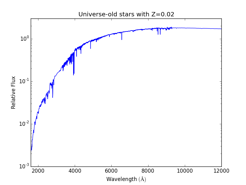
spec.write_out_SED(name="SED.out", flux_norm=5200)
Below is an example of an absurd SED for universe-old stars all with
solar metallicity at a redshift of zero. Note that even in this example,
a ds is required.
import yt
import numpy as np
from yt.analysis_modules.star_analysis.api import SpectrumBuilder

ds = yt.load("Enzo_64/DD0030/data0030")
spec = SpectrumBuilder(ds, bcdir="bc", model="chabrier")
sm = np.ones(100)
ct = np.zeros(100)
spec.calculate_spectrum(star_mass=sm, star_creation_time=ct,
                        star_metallicity_constant=0.02)
spec.write_out_SED('SED.out')
And the plot:
In this example below, the halos for a dataset are found, and the SED is calculated and written out for each.
import yt
from yt.analysis_modules.star_analysis.api import SpectrumBuilder
from yt.data_objects.particle_filters import add_particle_filter
from yt.analysis_modules.halo_finding.api import HaloFinder

def Stars(pfilter, data):
    return data[("all", "particle_type")] == 2
add_particle_filter("stars", function=Stars, filtered_type='all',
                    requires=["particle_type"])

ds = yt.load("enzo_tiny_cosmology/RD0009/RD0009")
ds.add_particle_filter('stars')
halos = HaloFinder(ds, dm_only=False)
# Set up the spectrum builder.
spec = SpectrumBuilder(ds, bcdir="bc", model="salpeter")

# Iterate over the halos.
for halo in halos:
    sp = halo.get_sphere()
    spec.calculate_spectrum(
        star_mass=sp[("stars", "particle_mass")],
        star_creation_time=sp[("stars", "creation_time")],
        star_metallicity_fraction=sp[("stars", "metallicity_fraction")])
    # Write out the SED using the default flux normalization.
    spec.write_out_SED(name="halo%05d.out" % halo.id)